Click a square on the Othello playground and a server on a single CPU core starts imagining the future. It grows a tree of positions, follows hundreds of promising lines through it, and answers with the move that those lines favour most. On the benchmark machine, 500 of those simulations take about a tenth of a second.
Two ideas make that possible, and both come from AlphaZero 1. A neural network looks at a board and says which moves deserve attention and who is winning. A tree search spends its effort where the network points. Neither idea is hard to state. Making them fast and strong enough for one core without a GPU is the engineering behind the engine.
Othello in brief
Two players, black and white, place discs on an 8x8 board. Black moves first from a starting position with four discs in the centre.
A move is legal when the new disc encloses at least one opponent disc. In one of eight directions (along a row, a column or a diagonal), the squares next to the new disc must hold one or more consecutive opponent discs, followed by a disc of the mover. Every enclosed opponent disc flips to the mover's colour. A player without a legal move passes, and the game ends when neither player can move. The player with more discs wins.
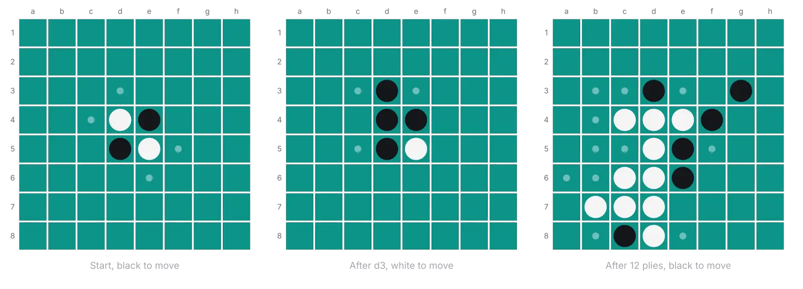
In each position, dots mark the squares where the player to move may play. The starting position offers four moves, the position after d3 leaves white three, and the position after twelve plies gives black eleven.
The rules fit in a paragraph, but the game grows quickly. From the starting position, the number of distinct move sequences of ten plies is already 24,571,284. A search cannot visit them all, so the engine has to choose which positions deserve its time, and it has to visit each of them cheaply.
Where a move spends its time
A move is the result of many small simulations, and every simulation repeats the same chain of work. It takes a position, finds the legal moves, plays one of them, asks the network how good the new position is, and records the answer in a tree. The cost of a move is the cost of that chain multiplied by the number of simulations, and each link of the chain offers its own room for improvement:
- The board. A position stored as a grid needs a loop over squares for every question, and the engine asks millions of questions per move. A representation that answers them with a few arithmetic instructions changes the price of every simulation.
- The network. The model judges the positions, so its design sets both the quality of the judgement and the cost of each evaluation. A smaller network is cheaper to run, and the training decides how much quality it keeps.
- The search. The tree decides which lines get simulations and remembers what the earlier simulations found. Its data structures and the order in which it evaluates leaves change how often the network runs and how much memory it touches.
- The hardware. The processor multiplies in wide vector instructions and reads memory through a cache hierarchy. Code that respects both runs several times faster than code that ignores them.
Board representation
Bitboards
A bitboard stores one bit per square, so a whole set of squares fits in one 64-bit integer. The position is two bitboards: one for the discs of the player to move and one for the discs of the opponent. Passing the turn swaps the two, and the network reads the same pair as its input, with the mover's discs as +1 and the opponent's as -1. One set of weights then plays both colours.
The figure shows a position and its two bitboards. Squares are numbered row by row, so the square in row and column is bit .
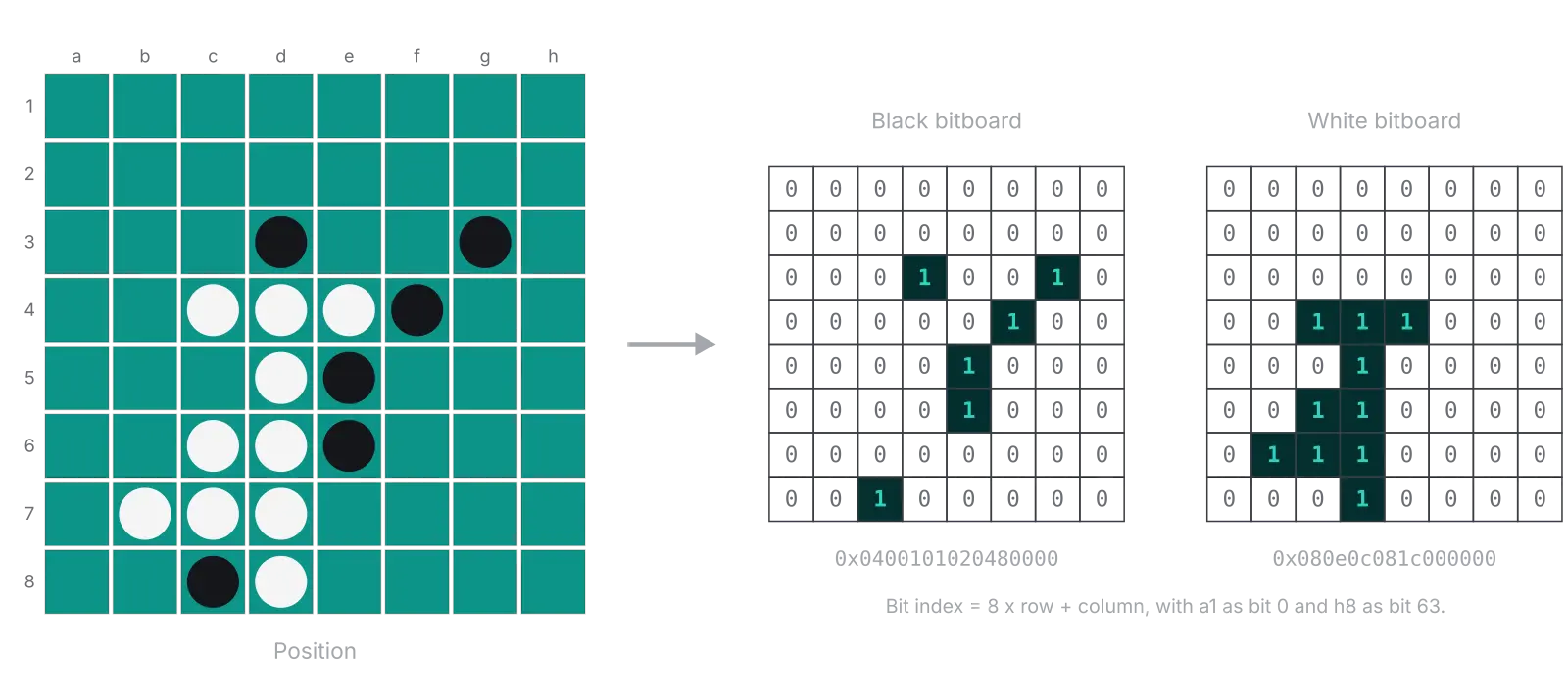
Shifting an integer moves every disc at once, and an AND with a mask clears the discs that left the board. Work that would loop over squares of an array turns into a few instructions on registers.
Move generation
By the rules, a square is a legal move when it is empty and, in at least one of the eight directions, the squares after it are one or more opponent discs followed by a disc of the mover. Checking this square by square takes a loop over 64 squares and 8 directions. With bitboards, one short sequence of operations finds the legal squares of the whole board for one direction at once.
The sequence works from the other end of the run: it starts at the discs of the mover and walks toward the empty squares. Two bitboards describe the position: holds the discs of the mover and the discs of the opponent. The set holds every other square, the empty ones. For a direction , moves every square of the set one square in that direction, and a square that would leave the board disappears. The legal squares for come from the following sets:
Each set has a meaning:
- is the set of opponent discs that touch a disc of the mover in the direction . Every run of opponent discs that the mover can use starts with one of these discs.
- adds to every opponent disc that follows a disc of in the direction . Each step extends every run by one disc, and a run that has ended stays as it is.
- shifts the finished runs by one more square and keeps the empty squares. An empty square right after a run of opponent discs, which itself starts at a disc of the mover, is a legal move.
Six sets are enough: a line has eight squares, and a run needs a disc of the mover at one end and an empty square at the other, so it holds at most six opponent discs. The legal squares of the position are the union of over the eight directions. The pass action exists when that union is empty.
The example takes the East direction on one row, with the squares a to h from left to right. The mover has a disc on c, the opponent has discs on d and e, and the squares a, b, f, g and h are empty. The figure follows the sets row by row, and the yellow squares are the members of each set:
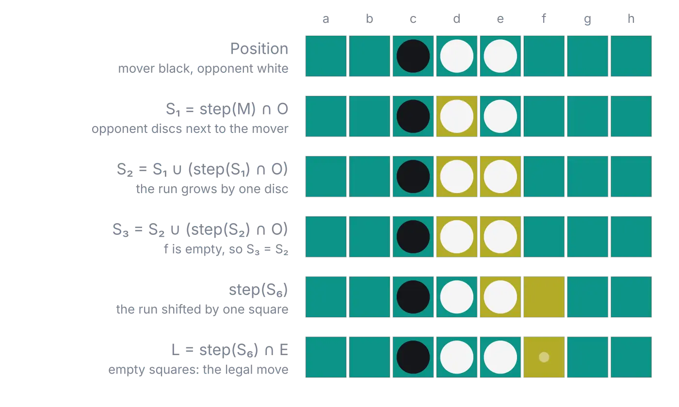
The table lists the same sets as bits:
| Set | Squares | Bits, a to h |
|---|---|---|
| c | 00100000 | |
| d, e | 00011000 | |
| a, b, f, g, h | 11000111 | |
| d | 00010000 | |
| d | 00010000 | |
| e | 00001000 | |
| d, e | 00011000 | |
| e, f | 00001100 | |
| d, e | 00011000 | |
| d, e | 00011000 | |
| e, f | 00001100 | |
| f | 00000100 |
In the third step, is empty and not an opponent disc, so the run stops at e and the later sets repeat . The result is the square f: a disc there closes the run d, e against the disc on c.
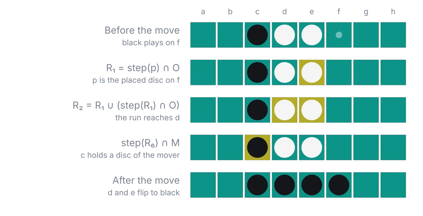
A move flips discs by the same procedure, started from the placed disc and ending at a disc of the mover. In each direction, the runs of opponent discs that start next to are collected with the same six steps, with in place of . The run flips only if the square after it holds a disc of the mover:
For = f and the direction West in the same row, is e, is d and e, and the next square, c, holds a disc of the mover, so d and e flip. A run that ends at an empty square or at the edge of the board does not flip.
The eight directions differ only in a shift amount and a mask that clears the bits that wrapped around an edge of the board:
| Direction | Bit shift | Edge mask removes |
|---|---|---|
| South | +8 | none |
| North | -8 | none |
| East | +1 | file A |
| West | -1 | file H |
| South-east | +9 | file A |
| North-west | -9 | file H |
| South-west | +7 | file H |
| North-east | -7 | file A |
A compiler sees both values as constants for each direction, so the generator becomes eight straight sequences of shifts, ANDs and ORs without a single branch.
The network
vAlpha3
The network is CNN_vAlpha3, the third version of the Alpha series of networks and the most
performant one.
It reads the canonical 8x8 board and produces two outputs: a policy over 65 actions (the 64
squares and a pass) and a value between -1 and 1 that estimates the outcome for the player to
move.
The deployed network uses 16 channels in the first convolution and 64 in the residual stack:
===================================================================================================================
Layer (type:depth-idx)                   Output Shape              Param #                   Mult-Adds
===================================================================================================================
CNN_vAlpha3                              [1, 65]                   --                        --
├─Sequential: 1-1                        [1, 16, 8, 8]             --                        --
│    └─Conv2d: 2-1                       [1, 16, 8, 8]             416                       26,624
│    └─GroupNorm: 2-2                    [1, 16, 8, 8]             32                        32
│    └─LeakyReLU: 2-3                    [1, 16, 8, 8]             --                        --
├─Conv2d: 1-2                            [1, 64, 8, 8]             1,088                     69,632
├─Sequential: 1-3                        [1, 64, 8, 8]             --                        --
│    └─Conv2d: 2-4                       [1, 64, 8, 8]             9,280                     593,920
│    └─GroupNorm: 2-5                    [1, 64, 8, 8]             128                       128
│    └─LeakyReLU: 2-6                    [1, 64, 8, 8]             --                        --
│    └─Conv2d: 2-7                       [1, 64, 8, 8]             36,928                    2,363,392
│    └─GroupNorm: 2-8                    [1, 64, 8, 8]             128                       128
│    └─LeakyReLU: 2-9                    [1, 64, 8, 8]             --                        --
│    └─Conv2d: 2-10                      [1, 64, 8, 8]             36,928                    2,363,392
│    └─GroupNorm: 2-11                   [1, 64, 8, 8]             128                       128
│    └─LeakyReLU: 2-12                   [1, 64, 8, 8]             --                        --
├─Sequential: 1-4                        [1, 1024]                 --                        --
│    └─Linear: 2-13                      [1, 1024]                 4,195,328                 4,195,328
│    └─LayerNorm: 2-14                   [1, 1024]                 2,048                     2,048
│    └─LeakyReLU: 2-15                   [1, 1024]                 --                        --
│    └─Dropout: 2-16                     [1, 1024]                 --                        --
├─Sequential: 1-5                        [1, 512]                  --                        --
│    └─Linear: 2-17                      [1, 512]                  524,800                   524,800
│    └─LayerNorm: 2-18                   [1, 512]                  1,024                     1,024
│    └─LeakyReLU: 2-19                   [1, 512]                  --                        --
│    └─Dropout: 2-20                     [1, 512]                  --                        --
├─Linear: 1-6                            [1, 65]                   33,345                    33,345
├─Linear: 1-7                            [1, 1]                    513                       513
===================================================================================================================
Total params: 4,842,114
Trainable params: 4,842,114
Non-trainable params: 0
Total mult-adds (Units.MEGABYTES): 10.17
===================================================================================================================
Input size (MB): 0.00
Forward/backward pass size (MB): 0.27
Params size (MB): 19.37
Estimated Total Size (MB): 19.64
===================================================================================================================
Three choices in this design carry most of its character. The residual shortcut lets information skip the convolutions, which helps a deeper stack train. Group normalization works on groups of channels, so it behaves the same for a batch of one board and a batch of sixty-four, which suits a network that trains in batches and serves single positions. LeakyReLU passes a small slope for negative inputs, so a neuron whose input turns negative still receives gradient.
The same architecture with 64 and 256 channels has 18,687,810 parameters. The deployed network is 3.86 times smaller.
Where the weights are
Almost all of the parameters sit in one layer. The first fully connected layer holds 86.7% of them, and the convolutional trunk holds 1.8%. The arithmetic is distributed differently:
| Layer | Multiply-adds |
|---|---|
| Entry convolution | 0.03 M |
| Shortcut | 0.07 M |
| Convolution 16 to 64 | 0.59 M |
| Two convolutions 64 to 64 | 4.72 M |
| FC 1 | 4.19 M |
| FC 2 | 0.52 M |
| Heads | 0.03 M |
| Total | about 10.2 M (20.3 MFLOP) |
The convolutions and the dense layers cost about the same amount of arithmetic, but the dense layers read about 50 times more weights. One half of the network is limited by how fast the processor can multiply, and the other half by how fast memory can deliver weights. That split decides how the network can be made fast on a CPU.
Search
Monte Carlo tree search
A game tree has a node for every position and an edge for every legal move. Monte Carlo tree search (MCTS) explores that tree selectively and never expands all of it 2. It repeats four steps 3:
- Selection. Walk down from the root, choosing a child at every node, until the walk reaches a node that has no children yet.
- Expansion. Create the children of that node, one for each legal move.
- Evaluation. Estimate how good the new position is. Classic MCTS plays random moves to the end of the game and uses the result. AlphaZero replaces that rollout with the value of a network 1.
- Backup. Walk back up the path and update the statistics of every node on it.
The choice in the first step decides the quality of the search. It has to exploit lines that look good and still explore lines that the search has barely tried. The engine scores each action with
Here is the average outcome of the earlier simulations that took action in position . The prior is the probability that the network assigned to the action. The visits of the position are counted by , and counts the visits of the action. The score rewards actions that did well so far, actions that the network likes, and actions that the search has barely tried. The last bonus shrinks with every visit, so the average outcome takes over once an action has collected enough evidence 13.
The network supplies the two missing ingredients. When expansion creates the children of a position, the policy of the network, limited to the legal moves and renormalized, becomes their priors . If the legal moves hold no probability at all, the priors are uniform. The value of the network becomes the result of the evaluation step, and a finished game uses its real result instead, with a draw counting as 0.0001. The backup flips the sign of the value at every step of the path, because the two players alternate.
When the simulations are done, the visit counts of the root decide the move. The engine plays the most visited move, and it breaks ties at random. The same counts, raised to the power and normalized, give a probability distribution over moves, which the playground shows as AI hints.
The exploration constant defaults to 1.5. Two optional schedules change it with the visit count of a position. Both use the factor and a floor of 0.5: the increment schedule starts at 0.5 and rises toward , and the decrement schedule starts at and falls toward 0.5.
Recognising positions
Different move orders reach the same position, so a search that treats every path as new would evaluate the same position again and again. The engine keeps one node for each position and finds it through a hash table. A node can then have several parents, and the structure is a directed acyclic graph and not a tree 2. Every path that reaches a shared node adds its simulations to the same statistics, and the network evaluates the position once.
The table needs a key that identifies a position. A hash function turns the position into a 64-bit number that is cheap to compute and the same for the same position. Zobrist hashing assigns a random 64-bit number to every combination of a square and a colour and combines the numbers of the occupied squares with XOR. Another choice mixes the two bitboards of the position directly with a 64-bit integer mixer. Two different positions can still land on the same number, so each table entry also stores the exact pair of bitboards and compares it on lookup. A collision then costs one extra comparison and never merges two positions.
Evaluating leaves in batches
A pass through the network reads every weight from memory, and that read costs more than the arithmetic. If the search hands the network four positions at a time, the weights are read once for the four.
So the search collects up to four leaves before it calls the network. The simulations of a batch walk down the tree one after another, and each one leaves a virtual loss on the edges of its path. A virtual loss makes those edges look slightly worse, so the next simulation of the batch takes a different route. Tree-parallel versions of MCTS use the same trick to keep several threads out of each other's way 2, and here it works inside a single thread. When the batch is full, one pass evaluates all new leaves, and the real values replace the virtual losses.
A batch of one is the plain sequential algorithm. The service uses a batch of four.
Anatomy of a search
The engine can export the tree that a search built. The pictures come from the C++ engine with the deployed network. A card is a position: a small board, the number of visits and the average outcome for black. The border of a card is orange when white is ahead and blue when black is ahead. A red ring marks the move that led to the position. Edges carry the move and its visit count, and the orange line follows the most visited move at every level. Each card lists how many moves it leaves out.
The opening
The first tree is a 400-simulation search from the starting position. It shows the three most visited moves at each of two levels.
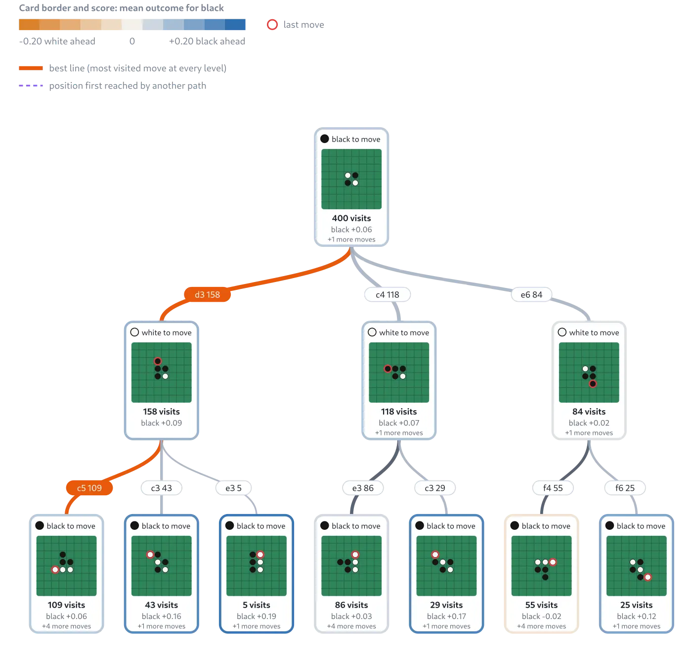
The starting position has four legal moves, and the symmetry of the board makes them equivalent. The network is not exactly symmetric, though, so the search does not treat them equally: d3 collects 158 visits, c4 118, e6 84, and the fourth move only 40. Training on rotated and mirrored boards teaches the network about symmetry without enforcing it, and a search amplifies the small differences that remain. All averages sit near zero (black +0.06 at the root), which fits a balanced opening.
Two routes to one position
The second figure is a 1,500-simulation search from the position after e6 and f4, with black to move.
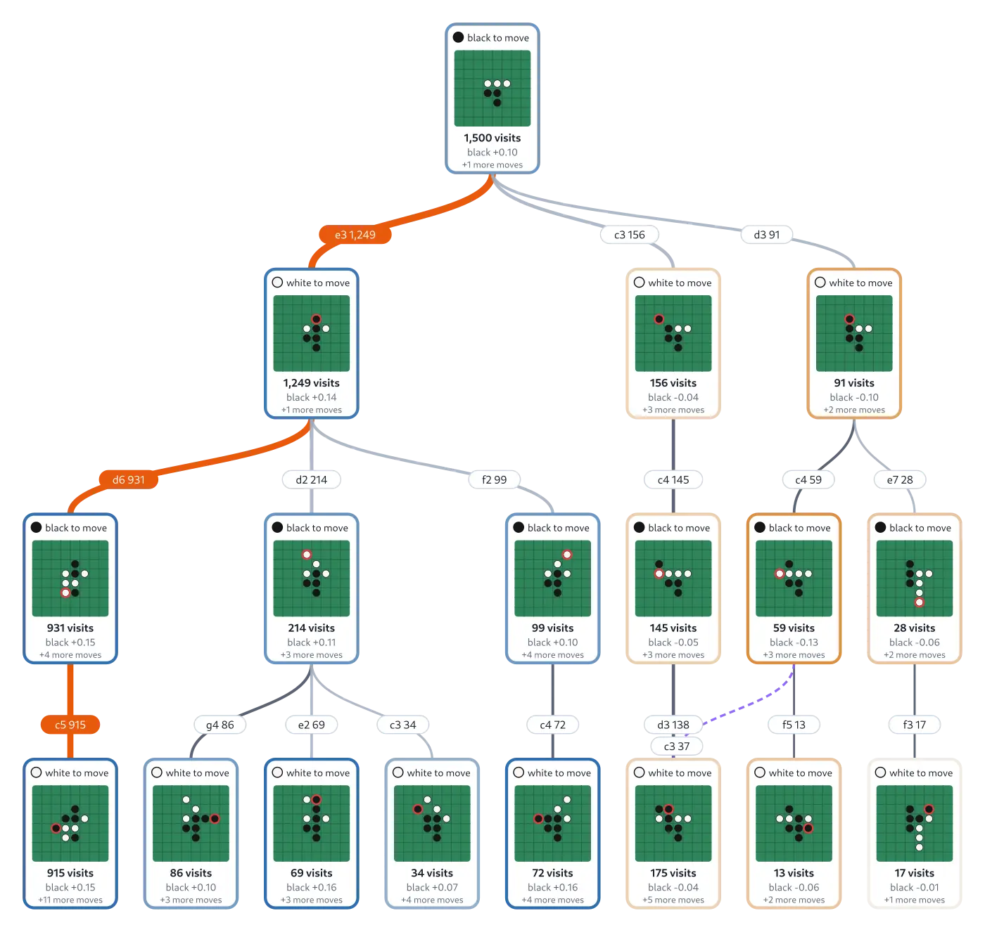
The dashed purple edge marks a position that the search had already reached by another route. Black plays c3, white c4 and black d3, or black plays d3, white c4 and black c3, and both orders end in the same position. That position has 175 visits: 138 came down the first order and 37 down the second. The network evaluated it once.
The endgame
The third tree is a 1,500-simulation search after 52 plies of a balanced game, with black to move.
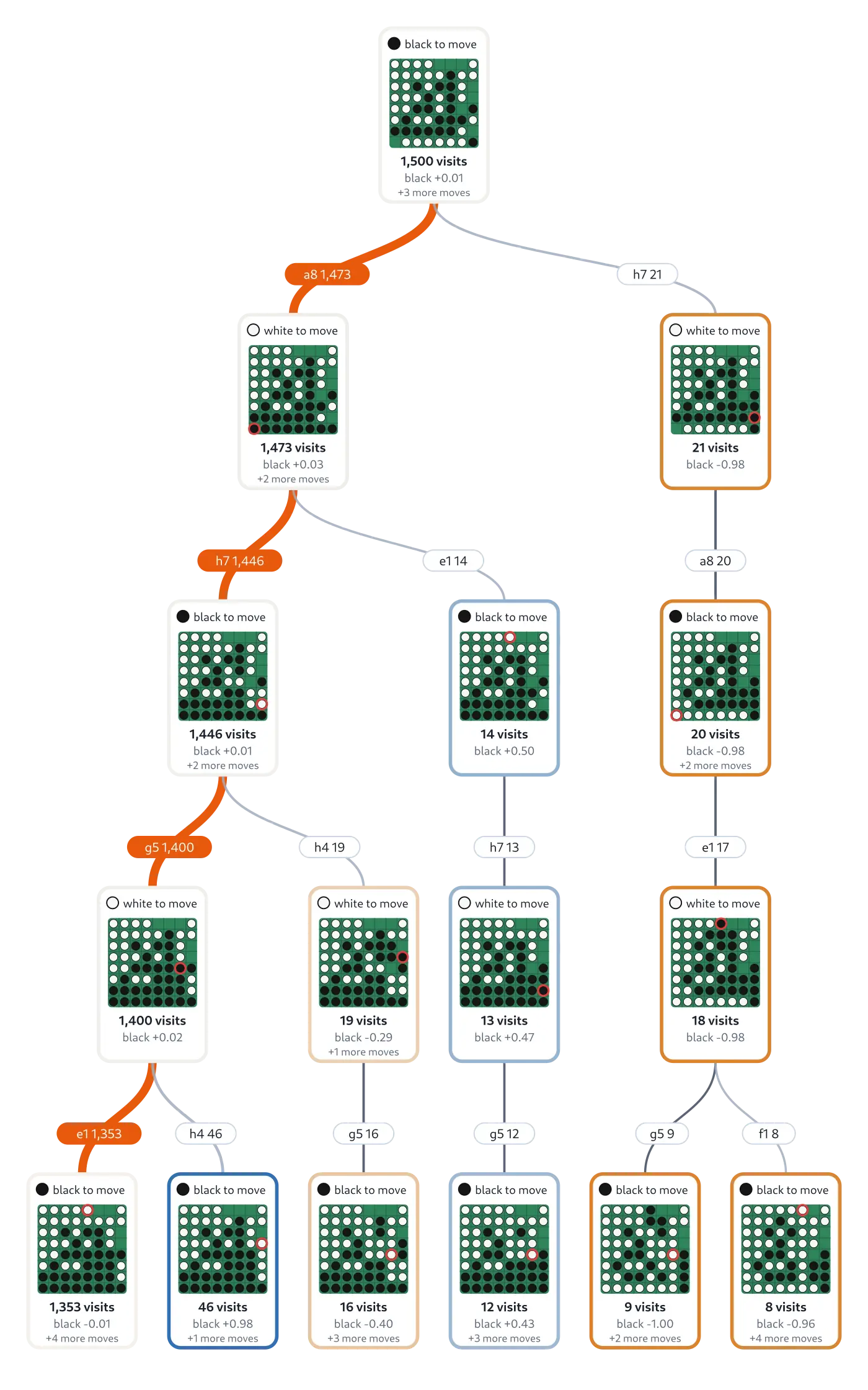
Few moves remain, and the search behaves accordingly. The root gives a8 1,473 of its 1,500 visits, and the average outcome along the best line stays between +0.01 and +0.03: the engine sees a balanced position and plays it out. The side branches are decisive. After h7 the value for black is -0.98 on only 21 visits, because the search finds a forced loss quickly and stops spending simulations there. Another branch shows +0.98 for black after an inaccurate white reply. Values that sit close to -1 or +1 on few visits are what a search close to the end of a game looks like.
Training
Self-play
The network learns by playing itself, and the recipe follows AlphaZero 1. The current network plays a game against itself and chooses every move with the search. For each move, the search turns its visit counts into a probability distribution and the engine samples the move from it. The sampling temperature decays exponentially with the move number, , so the opening explores and the endgame converges on the best move.
Every position of the game is stored with the visit distribution as the policy target. When the game ends, its result becomes the value target of each position, with the sign taken from the point of view of the player who moved there. Each position is stored in all eight symmetries of the square (four rotations, each with and without a mirror image), and the policy target follows the transformation. One game then yields eight times as many samples.
The network trains on a window of the most recent iterations with Adam (learning rate 0.001) on the sum of two terms:
The first term is the cross-entropy between the visit distribution and the policy output of the network, written . The second is the squared error between the game result and the value output of the network, written . AlphaZero minimizes the same two terms and adds an L2 penalty on the weights 1.
Arena gate
A new network must prove itself before the loop keeps it. After each training step, it plays a match against the previous network, half of the games with each colour, and both sides choose their moves with . If wins divided by wins plus losses falls below the update threshold, the previous weights come back and the new network is discarded. Otherwise the new network replaces the previous one and generates the data of the next iteration. A network that got worse never reaches the loop, and the next round of self-play starts from the last network that passed.
The trainer can also mix the move of an external solver, Egaroucid 4, into the policy target of some positions, so the network sees moves that self-play alone would not find.
Distillation
A network with 18.7 million parameters is more than one core can afford. Knowledge distillation trains a smaller student to reproduce a trained teacher. The repository's distillation notebooks 5 keep the architecture and shrink the convolutions. The student has the same layers with fewer channels, for example 16 and 64 instead of 64 and 256, and the deployed network has that shape.
The student never needs a game result and never runs a search while it learns. Each iteration it studies boards that come from random legal moves, together with the eight rotated and mirrored copies of each board, since the teacher answers any board it is asked about. A single forward pass of the frozen teacher provides the targets.
The policy loss compares the softened distributions of teacher and student on the legal moves, and the value loss compares the two value outputs:
Here and are the logits of the student and the teacher, is the softmax, and and are their values. The temperature softens both distributions. A softened distribution shows how the teacher ranks the moves it does not choose, and the student learns that ranking along with the favourite move. The factor keeps the size of the gradients comparable across temperatures.
A validation gate guards each iteration, like the arena gate does for self-play. The loss of the student on a held-out set of boards is recorded before the iteration trains, and if the iteration made that loss worse, the earlier weights return. The notebook trains with Adam at a learning rate of 0.001, ten epochs per iteration, batches of 64 and a temperature of 4, over 100 iterations of 1,000 boards each.
A second notebook adds Egaroucid 4 to the targets. For every training board it asks the solver for its move , puts extra probability mass on that move and renormalizes the teacher's distribution:
The student then matches with the same loss, and the value target still comes from the teacher alone. This notebook runs 20 iterations of 10,000 boards at temperature 2, with Egaroucid at level 5.
Evaluation
Two measurements compare the deployed network, alpha3S-v2.1, with two earlier checkpoints of the
same size (alpha3S-v2.0 and alpha3S-v1.0) and with the same architecture at 64 and 256 channels
(alpha-v3.0).
Both use the Python search with 500 simulations and , and PyTorch runs the
network on a GPU.
A third measurement compares search settings of the deployed network in the C++ engine.
Move prediction
The evaluation set holds 1,000,000 positions, each with a reference move. The measurement draws 2,000 of them at random (seed 42) and asks each network for a distribution over the 65 actions, once from the policy output alone and once from the visit counts of a search with . Top-k accuracy is the share of positions whose reference move is among the k most probable moves of the network. MRR is the mean of of the reference move. Macro F1 treats each move as a class and averages the F1 score over the classes. NLL is the mean negative log-probability of the reference move, and ECE is the gap between the confidence of the network and its accuracy over 15 confidence bins.
The raw policy:
| Network | Top-1 | Top-3 | Top-5 | MRR | Macro F1 | NLL | ECE |
|---|---|---|---|---|---|---|---|
| alpha3S-v2.1 | 41.0 | 75.3 | 88.2 | 0.605 | 0.409 | 2.129 | 0.233 |
| alpha3S-v2.0 | 39.7 | 74.4 | 88.3 | 0.597 | 0.402 | 2.053 | 0.202 |
| alpha3S-v1.0 | 36.2 | 71.3 | 86.1 | 0.567 | 0.363 | 2.201 | 0.225 |
| alpha-v3.0 | 35.0 | 69.4 | 83.7 | 0.554 | 0.345 | 2.224 | 0.268 |
The visit counts of a search with 500 simulations:
| Network | Top-1 | Top-3 | Top-5 | MRR | Macro F1 |
|---|---|---|---|---|---|
| alpha3S-v2.1 | 50.0 | 78.8 | 88.4 | 0.657 | 0.500 |
| alpha3S-v2.0 | 48.5 | 79.3 | 89.3 | 0.652 | 0.485 |
| alpha3S-v1.0 | 45.3 | 76.5 | 86.5 | 0.624 | 0.452 |
| alpha-v3.0 | 42.7 | 72.7 | 83.3 | 0.597 | 0.419 |
Accuracies are in percent.
The search raises top-1 accuracy by 8 to 10 percentage points for every network.
The deployed network has the highest top-1 accuracy with and without the search, and the 64/256
network has the lowest.
With 2,000 positions, a top-1 accuracy has a standard error of about 1.1 percentage points, so the
gap between alpha3S-v2.1 and alpha3S-v2.0 is within the noise of the measurement, and the gaps
to the other two networks are larger than it.
Games against Egaroucid
Egaroucid 4 plays as an external opponent at the search levels 1 to 5, with one thread and without its opening book. Each game starts from a random opening of four plies. The two games of an opening swap the colours, and the network chooses its moves from a search with 500 simulations and . Each network plays 20 games at each level.
Wins, draws and losses of the network:
| Network | Level 1 | Level 2 | Level 3 | Level 4 | Level 5 |
|---|---|---|---|---|---|
| alpha3S-v2.1 | 18-1-1 | 16-0-4 | 7-0-13 | 7-1-12 | 1-1-18 |
| alpha3S-v2.0 | 19-1-0 | 12-0-8 | 9-1-10 | 4-0-16 | 1-1-18 |
| alpha3S-v1.0 | 16-0-4 | 11-1-8 | 8-1-11 | 5-0-15 | 0-0-20 |
| alpha-v3.0 | 16-1-3 | 10-0-10 | 4-0-16 | 1-0-19 | 0-0-20 |
Mean disc difference at the end of a game, network minus Egaroucid:
| Network | Level 1 | Level 2 | Level 3 | Level 4 | Level 5 |
|---|---|---|---|---|---|
| alpha3S-v2.1 | +15.8 | +2.3 | -14.9 | -13.9 | -30.8 |
| alpha3S-v2.0 | +17.4 | -4.2 | -6.4 | -22.6 | -22.6 |
| alpha3S-v1.0 | +6.2 | -3.2 | -18.8 | -22.8 | -33.4 |
| alpha-v3.0 | +2.7 | -11.2 | -26.3 | -37.7 | -40.2 |
All four networks win most games at level 1, with 16 to 19 wins out of 20. The deployed network also wins 16 of 20 at level 2 and 7 of 20 at levels 3 and 4, and no network wins more than one game at level 5. At levels 3 and 4, the 64/256 network wins the fewest games of the four. With 20 games per level, a win rate has a standard error of up to 11 percentage points, so differences of a few games between two networks do not separate them.
Batched leaves
The service evaluates up to four leaves per network pass, and the virtual losses of a batch steer its simulations along different paths. This measurement compares the C++ search of the deployed network with a batch of four against the same search with a batch of one, with 500 simulations and .
The first comparison asks how often the move changes. It uses 2,000 random positions of 1 to 58 plies, and compares the most visited move of both searches. The last column is a reference: the same search with a batch of one and 1,000 simulations against 500.
| Positions | Same top move, batch 4 vs batch 1 | Same top move, 1,000 vs 500 simulations |
|---|---|---|
| 1 to 20 plies (723) | 97.8% | 93.8% |
| 21 to 40 plies (678) | 96.6% | 91.0% |
| 41 to 58 plies (599) | 96.7% | 97.7% |
| All (2,000) | 97.1% | 94.0% |
The mean total variation distance between the two visit distributions is 0.029 for batch 4 against batch 1, and 0.065 for 1,000 against 500 simulations. A batch of four changes the move in about 3% of the positions, which is less than doubling the number of simulations changes it.
The second comparison plays the two configurations against each other. Each match has 100 random openings of four plies, and each opening is played with both colours, for 200 games. The score counts a win as 1 and a draw as 0.5. The margin is the 95% interval of the score.
| Match | Batch 4 wins | Batch 1 wins | Draws | Batch 4 score |
|---|---|---|---|---|
| 500 simulations each | 81 | 105 | 14 | 0.440 ± 0.069 |
| Batch 4 with 500, batch 1 with 250 | 148 | 41 | 11 | 0.767 ± 0.059 |
With equal simulations, the batch of four scores 0.44, and the interval just reaches 0.5, so the loss of strength is small and the measurement does not settle it. The second match compares equal time: a batch of four with 500 simulations costs about as much as a batch of one with 250 (106 and 123 ms in the latency table), and it wins 148 games to 41.
Making the engine fast
The C++ engine rebuilds the rules, the network and the search around the hardware. The Python implementations of the same parts serve as the reference that its tests compare against. The benchmark scripts and the raw results are in the serving repository 6.
Rules
Medians on one pinned core:
| Operation | Python bitboard | C++ | Ratio |
|---|---|---|---|
| Legal moves | 12.5 to 18.8 µs | 7.7 ns | 1,600x to 2,400x |
| Play a move | 10.4 to 22.3 µs | 14.5 ns | 700x to 1,500x |
| Count ten plies | not measured | 0.51 s | 48.2 million positions per second |
The Python ranges cover the start, the middle and the end of a game, where a fuller board costs more. At these speeds the rules disappear from the profile of a search, and the network becomes the expensive part. A test plays random games through both implementations side by side and compares legal moves, next positions and results, and a second test counts the positions reachable in up to ten plies and compares them with the known totals.
Search layout
The Python search is recursive. Its statistics live in dictionaries keyed by a Zobrist hash of the board. At every node it loops over all 65 action slots and converts between numpy arrays and bitboards, and it calls PyTorch once per leaf. The C++ search keeps the algorithm and rebuilds the data layout:
| Aspect | Python search | C++ search |
|---|---|---|
| Node store | Dictionaries keyed by board hash | Open-addressing table from the position to a node index, with nodes and edges in contiguous arrays |
| Edge | Entries in four dictionaries | 16 bytes: prior, mean value, visits, child index |
| Selection | Loop over 65 action slots | Loop over the legal edges only, with and computed once per node |
| Control flow | Recursion | Explicit path stack |
| Evaluation | One PyTorch pass per leaf | Up to four leaves per pass |
| Randomness | numpy | xoshiro256** |
A test feeds both searches the same positions with a stub evaluator that returns deterministic pseudo-random policies and values. With a batch of one, the visit counts match exactly in all three schedules and across a sequence of moves with the tree kept. A second test compares the two engines with the trained network.
Weight format
An export script converts a PyTorch checkpoint into one binary file. The header holds a magic number, a format version and the layer shapes, and the tensors follow in the order the kernels read them. Convolution weights are stored per kernel tap with the input channels contiguous. Fully connected weights are stored in tiles of 16 outputs, aligned to 64 bytes. The two large fully connected matrices can be stored in half precision and converted when read. The loader validates the header and the sizes and rejects other format versions.
Kernels
- Padded feature maps. Feature maps live in buffers padded by the kernel radius, so the inner loops of the 3x3 and 5x5 convolutions need no bounds checks.
- Convolution microkernel. A block of four squares and sixteen output channels keeps eight vector accumulators in registers, broadcasts each input value and applies fused multiply-adds. One read of a weight serves four squares, and in isolation the kernel runs close to 80% of the measured multiply-add peak at about 4 GHz.
- Fused normalization. GroupNorm, LayerNorm and LeakyReLU run inside the layer that produces the data, and every buffer belongs to a preallocated per-thread scratch area, so an evaluation allocates nothing.
- Dense tiles. The 4096-by-1024 matrix takes 16.8 MB in fp32 and does not fit in the L2 cache. Each 16-output tile streams its weights while a software prefetch runs 192 inputs ahead of the multiply-adds.
- Several boards per pass. A pass applies the weights to up to four boards.
- Instruction set dispatch. The AVX2, FMA and F16C kernels run when the CPU reports those features, and a plain-loop implementation runs otherwise. The plain loops also serve as the reference of the tests, and the service logs which set it chose at startup.
The C++ network matches PyTorch within 1e-4 on logits and value with fp32 weights, on random and on real positions. With fp16 weights the tolerance is 2e-2.
Roofline analysis
The roofline model 7 bounds the performance of a kernel by two numbers: the peak arithmetic rate of the processor and the rate at which memory delivers data. A kernel that performs many operations on every byte it reads runs into the arithmetic limit first, and one that performs few runs into the memory limit. For a layer, that gives a floor for its time:
The benchmark measures both peaks on the pinned core and does not rely on datasheet values. The multiply-add peak has a median of 134.2 GFLOP/s, and 154.3 GFLOP/s at best. The read bandwidth depends on how much data is in play, because the caches serve small working sets and main memory serves large ones:
| Working set | Read bandwidth |
|---|---|
| 256 KiB | 166.6 GB/s |
| 2 MiB | 94.8 GB/s |
| 8 MiB | 53.2 GB/s |
| 16 MiB | 78.0 GB/s |
| 64 MiB | 33.9 GB/s |
| 512 MiB | 29.0 GB/s |
The floor of each layer for one board:
| Layer | Compute floor | Memory floor, fp32 | Memory floor, fp16 | Limit |
|---|---|---|---|---|
| Entry convolution | 0.38 µs | 0.01 µs | 0.01 µs | compute |
| Shortcut | 0.98 µs | 0.02 µs | 0.02 µs | compute |
| Convolution 16 to 64 | 8.8 µs | 0.2 µs | 0.2 µs | compute |
| Convolution 64 to 64, each of two | 35.2 µs | 0.9 µs | 0.9 µs | compute |
| FC 1 | 62.5 µs | 215.1 µs | 157.7 µs | memory |
| FC 2 | 7.8 µs | 22.1 µs | 11.1 µs | memory |
| Heads | 0.5 µs | 1.0 µs | 1.0 µs | memory |
| Sum of the floors | 318.7 µs | 250.2 µs |
One layer dominates. For a single board, FC 1 accounts for two thirds of the fp32 floor, and its time is the time to read its weights. Three decisions follow from that table: tiles with prefetch for the weight stream, half-precision weights that cut the memory floor of FC 1 by 27%, and batches of four boards that pay the 215 µs read once for four boards.
Measured times
One board per call on one pinned core, with the median of 30 samples from six interleaved rounds.
The hardware counters come from perf stat, and the roofline share is the sum of the floors
divided by the measured time.
| Variant | Median per board | IPC | GFLOP/s | Roofline share | Speedup vs PyTorch, default threads | Speedup vs PyTorch forward, one thread |
|---|---|---|---|---|---|---|
PyTorch predict, default threads |
2,706.7 µs | 1.0x | ||||
PyTorch predict, one thread |
771.3 µs | 1.83 | 3.5x | |||
PyTorch forward, one thread |
684.3 µs | 1.84 | 4.0x | 1.00x | ||
| C++ plain loops, fp32 | 5,347.3 µs | 4.25 | 3.8 | 6.0% | 0.5x | 0.13x |
| C++ plain loops, fp16 | 8,040.7 µs | 5.40 | 2.5 | 3.1% | 0.3x | 0.09x |
| C++ AVX2, fp32 | 417.5 µs | 1.75 | 48.6 | 76.3% | 6.5x | 1.64x |
| C++ AVX2, fp16 | 285.8 µs | 3.23 | 71.0 | 87.5% | 9.5x | 2.39x |
| C++ AVX2, fp32, four boards per call | 200.4 µs | 3.70 | 13.5x | 3.41x | ||
| C++ AVX2, fp16, four boards per call | 199.6 µs | 3.75 | 13.6x | 3.43x |
The four-board rows show the time per board. The PyTorch default-thread row varies by 22% between samples, and the pinned rows stay below 2%. The plain-loop rows are the portable reference that the tests compare against, and nobody tuned them.
With fp32 weights the AVX2 kernels reach 76% of the roofline floor. The remaining 24% is the work that the floor leaves out: normalization, activation functions and the writes between layers.
Half-precision weights bring one board down from 417 to 286 µs, because the dense layer reads half the bytes. The kernel then runs at 71 GFLOP/s, 53% of the arithmetic peak.
With four boards per call, both precisions need about 200 µs per board. The weight read is shared by four boards, so arithmetic limits the pass, and the cost of converting fp16 cancels what it saves on reads. That pass runs at 101 GFLOP/s, 75% of the measured peak, with an IPC of 3.70.
Latency of a move
The search benchmark times one call from an empty table on the same boards for every engine. It uses five boards in each of three regions (start, middle and end of a game) and reports the mean. The Python engine runs PyTorch with one thread on the pinned core, and all engines use the same network. Mean milliseconds per move:
| Region | Simulations | Python | C++, batch 1 | C++, batch 4 | Batch 4 vs Python |
|---|---|---|---|---|---|
| Start | 100 | 109.2 | 48.8 | 21.6 | 5.1x |
| Start | 500 | 572.7 | 233.6 | 106.5 | 5.4x |
| Start | 1,000 | 1,166.9 | 413.1 | 208.6 | 5.6x |
| Start | 2,500 | 3,064.2 | 1,027.3 | 505.4 | 6.1x |
| Middle | 500 | 578.9 | 203.9 | 101.0 | 5.7x |
| Middle | 2,500 | 3,198.3 | 1,017.7 | 500.9 | 6.4x |
| End | 500 | 160.1 | 25.7 | 18.8 | 8.5x |
| End | 2,500 | 624.1 | 43.2 | 34.2 | 18.3x |
At 500 simulations in the start region, the batched C++ search spends 213 µs per simulation. A four-board network pass costs 200 µs per board, so the network accounts for nearly all of it, and the tree work of selection, hashing and backup takes the remainder. Batching the leaves makes the search 2.2 times faster than the sequential C++ search there, because the time per board in the network falls from 417 to 200 µs and the rest stays the same.
The end of a game is cheap: 2,500 simulations take 34 ms. Few moves are legal, and the search keeps reaching finished games, which need no network.
Serving
The backend is a FastAPI application.
/move returns the engine's move for a board, a player and the search settings.
/hints returns the move distribution that the interface shades, and /health reports whether
the model is loaded.
One request makes one call into the C++ engine. The call releases the Python global interpreter lock, runs the whole search and returns a 65-element probability vector, so the interpreter stays out of the search loop.
A multi-stage Docker build compiles the extension and exports the weights in its first stage.
The runtime image holds numpy, FastAPI, the extension and the weight file, and it ships without
PyTorch.
The service runs on Cloud Run with one vCPU and 512 MiB.
The fp32 weights take 19.4 MB, and the search clears its tree when it grows past 200,000 nodes.
At startup the service logs which engine it runs, which instruction set the network uses (avx2
or scalar, with a warning for the second) and the batch size.
If the extension fails to import, the service starts the Python engine and logs the reason.
Limitations
- Every number comes from one core of one machine. The production CPU has a different cache hierarchy and clock, so its ratios between the variants can differ.
- The comparison of batch sizes covers one network, 2,000 positions and 200 games per match.
- The search benchmark samples five boards per region.
- The move-prediction measurement uses 2,000 positions and the games use 20 per level and network, so the differences between close networks fall within the noise.
Footnotes
-
D. Silver et al. A general reinforcement learning algorithm that masters chess, shogi, and Go through self-play. Science, 362(6419), 1140-1144, 2018. doi:10.1126/science.aar6404 2 3 4 5
-
C. Browne et al. A Survey of Monte Carlo Tree Search Methods. IEEE Transactions on Computational Intelligence and AI in Games, 4(1), 1-43, 2012. doi:10.1109/TCIAIG.2012.2186810 2 3
-
S. Taha. Understanding PUCT in Monte Carlo Tree Search. Documentation of the training repository. docs/mcts.md 2
-
T. Yamana. Egaroucid, an Othello AI. github.com/Nyanyan/Egaroucid 2 3
-
S. Taha. Knowledge distillation notebooks of the training repository: distill.ipynb and eg_distill.ipynb.
-
S. Taha. Serving repository with the C++ engine, the benchmark scripts and the results. github.com/systems-resarch-at-iba/othello
-
S. Williams, A. Waterman, D. Patterson. Roofline: An Insightful Visual Performance Model for Floating-Point Programs and Multicore Architectures. Technical Report UCB/EECS-2008-134, University of California, Berkeley, 2008. EECS-2008-134
